How to use
This page provides examples of how to use mapflow for creating animations and static plots.
Animating a DataArray
The main function of mapflow is animate, which creates a video from a 3D xarray.DataArray with time as the animation dimension.
import xarray as xr
from mapflow import animate

ds = xr.tutorial.open_dataset("era5-2mt-2019-03-uk.grib")
animate(da=ds['t2m'].isel(time=slice(120)), path='animation.mp4')
Notes:
Only two of
fps,upsample_ratio, anddurationcan be provided at the same time.Use
crfto control video quality (lower values mean better quality).Use
video_widthto control the output video width in pixels.Use
pad_inchesto set the padding (inches) around saved frames. Defaults to 0.2.
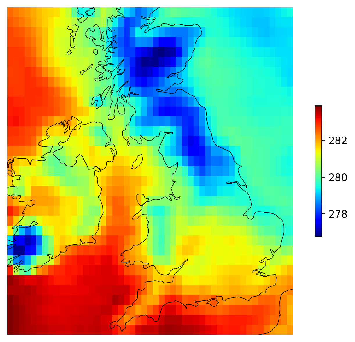
Creating a static plot
mapflow also provides a simple way to create static plots of 2D xarray.DataArray objects using the plot_da function.
import xarray as xr
from mapflow import plot_da

ds = xr.tutorial.open_dataset("era5-2mt-2019-03-uk.grib")
plot_da(da=ds['t2m'].isel(time=0))
Quiver plots
You can also create quiver plots to visualize vector fields. The plot_da_quiver function takes two xarray.DataArray objects representing the U and V components of the vector field.
import xarray as xr
from mapflow import plot_da_quiver

ds = xr.tutorial.load_dataset("air_temperature_gradient").isel(time=0)
plot_da_quiver(u=ds["dTdx"], v=ds["dTdy"], subsample=4)
Similarly, you can create quiver animations using the animate_quiver function. Provide 3D DataArrays with time as the animation dimension.
import xarray as xr
from mapflow import animate_quiver

ds = xr.tutorial.load_dataset("air_temperature_gradient")
animate_quiver(u=ds["dTdx"], v=ds["dTdy"], path='quiver_animation.mkv', subsample=3)
Advanced Usage: PlotModel and Animation classes
For more control and efficiency when creating multiple plots or animations of the same geographic domain, you can use the PlotModel and Animation classes directly. These classes pre-compute geographic borders, which can save time.
Using PlotModel:
import xarray as xr
from mapflow import PlotModel

ds = xr.tutorial.open_dataset("era5-2mt-2019-03-uk.grib")
da = ds["t2m"].isel(time=0)

p = PlotModel(x=da.longitude, y=da.latitude)
p(da)
Using Animation:
import xarray as xr
from mapflow import Animation

ds = xr.tutorial.open_dataset("era5-2mt-2019-03-uk.grib")
da = ds["t2m"].isel(time=slice(120))

animation = Animation(x=da.longitude, y=da.latitude, verbose=1)
animation(da, "animation.mp4")
Key Features
mapflow is designed to be intuitive and requires minimal user input. Here are some of the key features that make it easy to use:
Automatic Coordinate Detection:
mapflowautomatically detects the names of the x, y, and time coordinates in yourxarray.DataArray. If it fails to find them, you can specify them using thex_name,y_name, andtime_namearguments.Automatic CRS Detection: The library automatically tries to determine the Coordinate Reference System (CRS) from your data. If no CRS is found, you can pass it directly using the
crsargument.Robust Colorbars:
mapflowgenerates a colorbar that is robust to outliers by default, using the 0.01 and 99.9 quantiles. You can also customize the colorbar using thevmin,vmax, andcmaparguments, or even pass a custom matplotlib.colors.Normalize object via the norm argument.Integrated World Borders:
mapflowincludes a built-in set of world borders for plotting. If you need to use custom borders, you can provide them as ageopandas.GeoSeriesorgeopandas.GeoDataFrameusing thebordersargument.One-line Alternative to Cartopy: The
plot_dafunction provides a simple, one-line alternative to creating maps withcartopy, making it quick and easy to visualize your geospatial data.Flexible Output: Animations can be saved in various formats, including .mp4, .mkv, .mov, and .avi.
Parallel Processing: Frame generation for animations is done in parallel to speed up the process. You can control the number of parallel jobs with the n_jobs argument.